This is post is updated on 2022/12/20 to correct a couple statements below based on the Linkedin discussion we had and add an example of commit timing.

I remember reading

Using a parallel data processing regime/framework, TM1 can load upwards of 50.000 records per second per CPU core. In a 16 CPU core context, this can mean an overall data-load/update speed of roughly 800.000 records per second or 1 Billion records in 21 minutes!

in “Parallel Data Processing with IBM Planning Analytics” whitepaper by Andreas Kugelmeier (worth reading) a while back when I was writing about large scale TM1 models and thinking:

• surely that’s wishful arithmetics, no way you get to this kind of speed
• you shouldn’t be doing that kind of processing in PA, there are other systems better suited for the task

I have since participated in building a system that processes data on the similar scale (1.2 bln cells in 45 minutes) and it has been in production for about a year, so I thought it’s worth sharing some of the learnings.

Why so much data

This is labour forecasting for a large retail chain, so we calculate effort by:

• store - >1 thousand
• task - about a couple thousand different tasks in store
• day of week
• 15 minute interval in day
• about 10 measures

which ends up being 450m cells populated on average calculation run. And we have multiple versions that are ran in parallel.

Pic or didn’t happen:

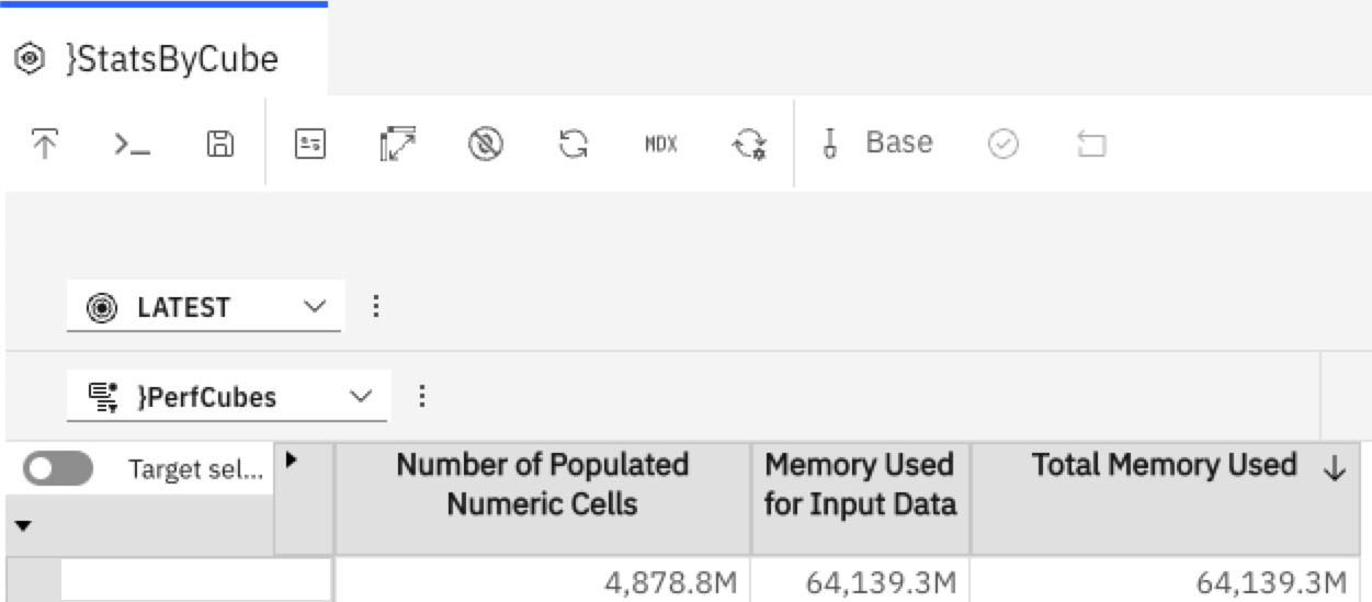
a typical day with ~7 different versions populated for the calculation.

How and some learnings

Some additional notes to my earlier ramblings on TI performance (NB: all still applicable):

• Running a bunch of TI’s in parallel as we’ve talked about before, but with RunProcess instead of runti. Still files for semaphores.
• Minimum amount of rule calculations on this scale and no N-level rules or feeders on such large cubes. We were using rules originally for a part of calculation and hoping that MTQ will handle scaling, but turns out it doesn’t. This challenged my usual ‘rules / processes’ prefernce.
• Since it’s a complicated calculation that users have to ‘trace’ frequently (that’s where rules were helpful before we removed them), we implemented a trace utility (essentially an Asciioutput for every calculation line in TI & an email with details to user asking for a trace), making processes looks like this:

...
  nRawMinutes =  nTimeValueByNumberOfTimes \ nLabourStandardtotalNumberSlotsPerDay;
  sDebugString = Expand('nTimeValueByNumberOfTimes (%nTimeValueByNumberOfTimes%) \ nLabourStandardtotalNumberSlotsPerDay (%nLabourStandardtotalNumberSlotsPerDay%)');
...
if (pTraceFile @<>'');
  AsciiOutput(pTraceFile, vSite,vTask,vDay,vTimeOfDay,'Raw Minutes', NumberTostring(nRawMinutes) ,sDebugString);
endif;
...

turned out to be useful

• We are doing multi-step allocation / distribution in this calculation, so there’s a lot of reading data committed by previous processes (steps of calculation). I couldn’t find a way to reliably identify the ‘previous processes has committed’ and have to rely on Sleeps instead. See section on commit timing below
  • It pained me no end, but there’s no way to detect a commit (update 2022/12/20: this is possible in REST Api, but not inside of PA / TIs at this point in time, hopefully we’ll get it in v12). I.e. you can detect that Process A has completed (Epilog tab finished), but not the Commit step of it that starts right after execution is finished to write data so it’s visible to other users or processes
  • Since we’re committing large data volumes (10s of millions of cells), commit takes a 5-10 seconds, just enough for the parallel framework to slip it through every now and then, start the following process and cause a ‘intermittent’ bug where some data wouldn’t be read correctly
  • I tried a ‘write to a small status cube once writing to big one is complete’ approach to detect commits, but PA treats both writes as different transactions in same TI, so a small cube is committed prior to the big one, duh
  • trying to read the data from the ‘big cube’ you’re writing to introduces unacceptable performance penalty (locking and memory growth to present you a readable view)
• ( update 2022/12/20 : looks like it’s a limitation of the code we’ve built, there are examples of scaling way past 24 threads that people mentioned on Linkedin, disregard the following and perform your own testing ) It looks like that there’s an internal product limit of how many threads can be accessing the same cube at the same time. And the magic number is somewhere around 16-20 threads, adding more threads (even if you have CPUs to spare) slows down processing. I.e. we run the 450m cells calculation in 45 min on 8 cores, can run 2 calculations of 450m in parallel (taking 16 cores) and still it’ll be 45 min, but adding a 3rd one will slow us back down to over the hour. Or on a single run 8 cores => 45 min, 16 cores => 30 min, 24 => more than an hour. Mystery :)
• current calculation runs 26k cells / s per core which is very close to my 30k/s target

Should PA be used for this

Back to the headline question - should this be done in PA at all?

I was constantly asking myself that during the implementation (and especially while debugging) and then had a chance to listen to the product owner’s demonstration of the system to the wider audience. Surprisingly enough this calculation wasn’t even mentioned, but the lot of more ‘standard’ PA pieces that we built around it (i.e. driver based calculations, scenario modeling, top-down adjustments) were really life-changing. None of them would’ve worked or be possible without that base calculation and PA was really well suited for doing those.

Using another system to do the calculation (Spark is the obvious candidate I kept thinking about) and building the required data integration out of PA and back in probably would’ve landed us in the same run time with added complexity of maintaing 2 systems.

And the very same calculation in the actual time tracking system is taking over 15 hours, so our 45 minutes seems like a good outcome at the end of the day.

Commit timing

Picture worth a 1000 words? 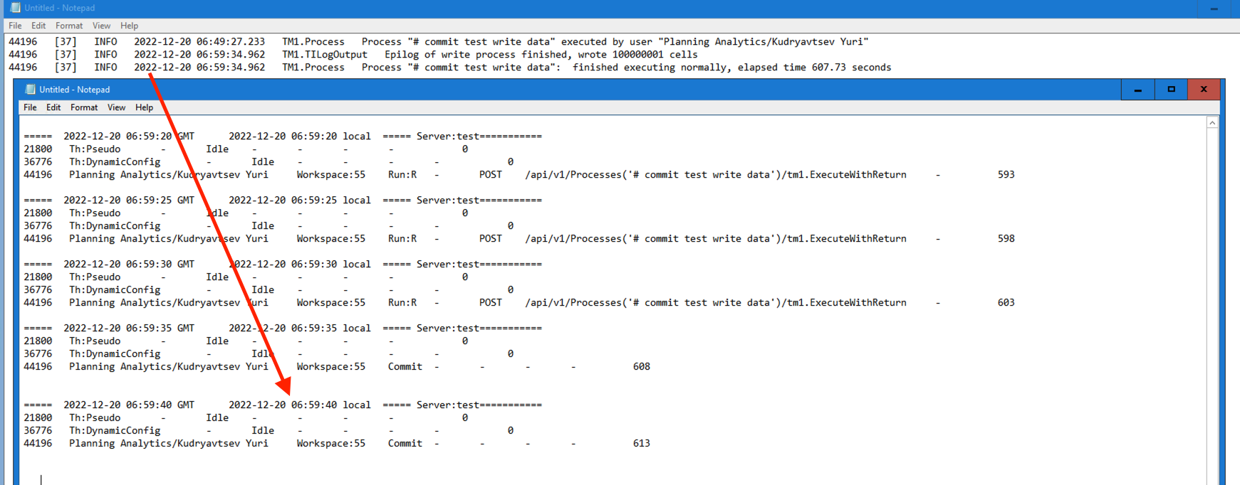tm1server.log (and any ExecuteProcess used in queue orchestration within TI) thinks the process is finished, whereas data is still committing for another 10 seconds (that’s running it with 100m records to write). Hence the need to Sleep to write committed data.

REST API correctly records the full execution time with Commit being a different section, but it requires you to ‘orchestrate’ TI runs outside of PA.

Here’s the sample code that you can use to reproduce it yourself (you’d need 1GB spare memory in you want to write 100 m cells as I did to see a ‘long commit’).

Process 1. Create test objects

Prolog

# Let's create a cube with 4 dimensions with 1000 elements each to write data to 
j = 1;
while (j<=4);
  sDim = 'CommitTest Dimension ' | NumberToString( j );
  DimensionCreate( sDim );
  i = 1;
  while (i<=1000);
    sElement = 'Element ' | NumberToString( i );
    DimensionElementInsert( sDim, '', sElement, 'N' );
    i = i + 1;
  end;
  j = j + 1;
end;

CubeCreate('CommitTest','CommitTest Dimension 1','CommitTest Dimension 2','CommitTest Dimension 3','CommitTest Dimension 4');

Process 2. Write data

BTW, this TI writes 100 m cells in 615s on PAoC – about 160k cells / s :)

Prolog

#let's loop through dimensions and populate cells until we reach the target number
#we have 4 dims 
CellPutS('NO','}CubeProperties','CommitTest','Logging');

CubeClearData( 'CommitTest' );
nDimSize1 = Dimsiz('CommitTest Dimension 1');
nDimSize2 = Dimsiz('CommitTest Dimension 2');
nDimSize3 = nDimSize3;
nDimSize4 = nDimSize4;

i = 1;
while (i<= pNumberOfCellsToWrite);
  nCoord1 = Mod(int(i/(nDimSize4*nDimSize3*nDimSize2)), nDimSize1) + 1; 
  nCoord2 = Mod(int(i/(nDimSize4*nDimSize3)), nDimSize2) + 1;
  nCoord3 = Mod(int(i/nDimSize4), nDimSize3) + 1;
  nCoord4 = Mod(i, nDimSize4) + 1;
   CellPutN(1000 * Rand(),
            'CommitTest',
            'Element ' | NumberToString(nCoord1), 
            'Element ' | NumberToString(nCoord2),
            'Element ' | NumberToString(nCoord3),
            'Element ' | NumberToString(nCoord4));

  i = i + 1;
end;

CellPutS('Yes','}CubeProperties','CommitTest', 'Logging');

Epilog

LogOutput( 'info', 'Epilog of write process finished, wrote ' | NumberToString(i) | ' cells' );

Process 3. Destroy test objects

Prolog

CubeDestroy( 'CommitTest' );
DimensionDestroy( 'CommitTest Dimension 1' );
DimensionDestroy( 'CommitTest Dimension 2' );
DimensionDestroy( 'CommitTest Dimension 3' );
DimensionDestroy( 'CommitTest Dimension 4' );