This post is an outline of the presentation I did at our internal knowledge share session recently. There’s no new or ground-breaking stuff here, just a review of well-known ideas and some of my takes on them.

The magic number

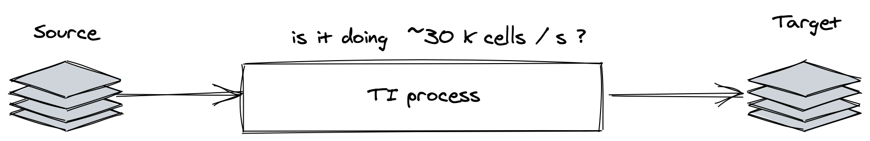
Whenever I’m looking at a TI performance, I start by carefully unrolling my trusted measuring tape that has only 1 line on it – at 30k records per second. It’s pretty worn out as this number hasn’t changed much since version 9.4 when I first saw TM1, but hey, I like it boring. Just in case you’re as bad in maths as I am: 30k per second is about 1.8 million per minute or 108m per hour.

30,000 records per second in a processing tab is around the absolute maximum of what I expect in terms of TI speed. So I think of a TI like this (yay simple):

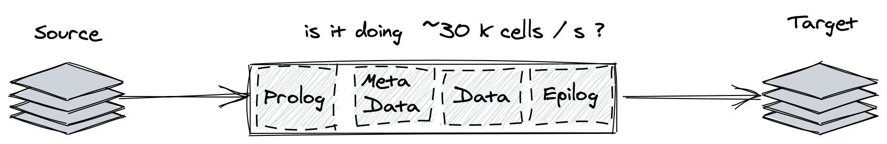
TI processing time total is a sum of time we spent on each tab:

• Prolog - you usually set up your source and done the pre-load cleanup here or do all the processing here
• Metadata - managing dimension hierarchies
• Data - loading data
• Epilog - post processing cleanup and potentially some data processing as well (please be careful if you’re doing anything with dimensions in epilog and generally don’t)

I’ll focus on data processing TIs for the sake of simplicity as dimension updates are a bit different in nature and less of a source of performance drama generally.

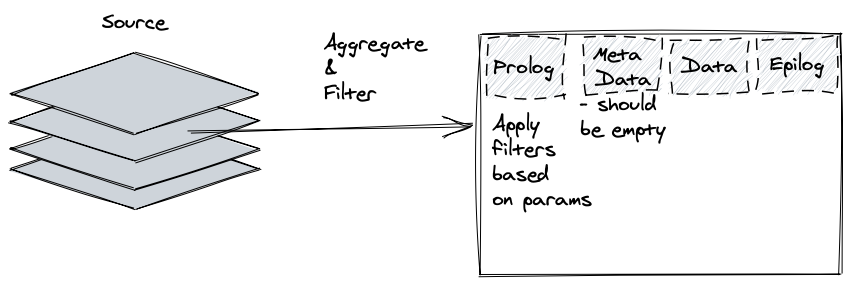
A good rule of thumb is that it’s best to separate dimension and data maintenace TIs and ideally run them in separate ‘commit sessions’ (different sections in multi-commit chore or different chores, runtis). So if you see something on both metadata and data tabs and it’s not just a dimension update TI – start thinking about splitting the dimension update part to a separate process to decrease locking (dimension updates lock related objects and data update TIs don’t) and improve performance. And, yeah, metadata and data read the same source data from scratch, so you improve performance by skipping Metadata section by going through source only once. I recently saw a 30 minute process that had record counting boiler plate code left in metadata tab, so removing that decreased processing time significantly.

To calculate the number of processed records / divide by time we spent in the process, we need to see where we’re doing the processing and then increment a counter for each data point we go through. Add something like nCountRecords = nCountRecords + 1 in Data tab and for each processing cycle in Prolog or Epilog.

So let’s say you get a number of X records per second:

• above 10000 – I would assume that anything in terms of what this process does is amazing and would focus on whether we can change the volume of source data it processes
• for anything below a 1000 – I’d definitely be interested to see what’s happening in the process that causes it to slow down

Decreasing the source volume

So we have a fast enough calculation pipe, how can we make it do less? There’s a few ways and I’ll list them from my most to least favourite one.

Read only the data you need

If you see a lot of ItemSkips or CellIncrementNs – there’s some potential for filtering or aggregation.

If your source is SQL – make sure you’re doing all the possible aggregations and filtering in that SQL query, databases are really built for this. And only read the data you need, having more columns in the query that you’re grouping by, but ignoring the columns in the TI itself can make TI read a lot more data than required. Ditto fitlering, if you’re seeing something like

If (month < X);
	Itemskip;
Endif;

it might be worth checking whether the month < X can be part of your SQL query.

If you’re reading a cube view, make sure you’re getting the level of consolidations you need, there’s usually little reason to sum leaf cells again to arrive at the same result. It might be worth creating special consolidations for reading data to decrease source volume, you can safely assume that consolidation is 100x faster than reading source data and CellIncrement’ing. I generally don’t like CellIncrements, in case you haven’t noticed before :)

A less well trodden path is using some assumptions of what data is ‘significant’ enough. This is especially interesting in allocation processes as you often end up splitting hairs up to lowest possible precision (e-14) that usually is quite frankly meaningless for any analysis. On one of the recent projects we made a set of ‘floor assumptions’ on the level of data that is ‘worth keeping’ and aggregated all the cells below these assumptions into a set of special placeholder coordinates to condense the dataset and improve performance by an order of magnitude without affecting the total values and with a tolerable loss of precision.

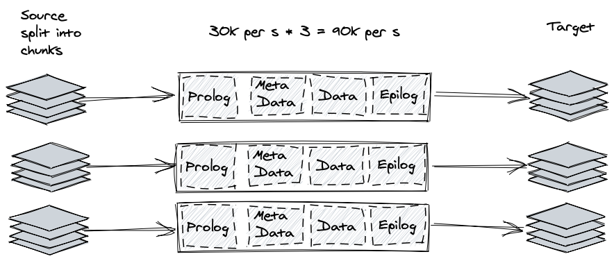
Run multiple versions of the same process in parallel

If you exhausted all the optimisation avenues within the TI and there’s no way to limit source, you can try decreasing it by splitting it against some dimesnion and running mutliple copies of the same TI in parallel.

There’s a ton of information out there on how to build TI parallel frameworks, I’ll just note the 2 main challenges you’d be facing when you embark on the journey (insert a joke about having 2 problems: performance and parallel processing framework).

Challenge 1:

What do we want?
Now
When do we want it?
Less race conditions

You need to know when processes start and finish and TM1 at the moment has a built in capability to asynchroniusly call an execution thread RunProcess(), but has no built capability to know if it ended or how did it end. So you need to build your own synchronisation mechanism using either files or cubes and spend a bit trying to ensure it’s watertight.

Challenge 2 of parallel processing in TM1 goes as follows:

What do we want?
No locking
When do we want it?
…
…
…

You need to be extra careful with using parallel processing frameworks as your your solution becomes a lot more exposed to any potential locks, therefore monitoring and exhaustive logging are paramount. Moreover, locks can be very gradual and tricky, I was recently dumb-founded by a lock that was triggered by an rule-driven alias that was added after the parallel processing framework was put together in a seemingly unrelated small dimension. There’s a long list of things that cause locks in TM1 that merit their own post(s?) and this list changes with server releases, so my approach is that the moment you use parallel frameworks you’d get locks, so you need to have logs to trace them.

I wrote about this before. The only way I haven’t seen work queue implemented so far is via a database and as a dutabase guy I’d be keen to try it out, having an append-only queue table should be very good for tracing execution and would enable some reporting straight of that table.

Read only changed data / Incremental processing

Another way to ‘read less’ is to try to only process the source data that has changed since the last time we ran the process. You need a way to identify ‘what changed’ between the runs and doing this reliably is the main challenge of this approach. I had success with using a static ‘as of last run’ copy of some of the key parameters that I would know change the calculation results, for example if contract dates and conditions didn’t change there’s no need to reprocess it again. Copying as of last run to static and using a consolidation of ‘current - as of last run’ is a common way to give you a list of ‘changed’ elements to use as source.

The main challenge in this approach is the added complexity of making sure that you know what kind off changes should trigger re-processing and spending time ironing the cases when this knowledge proves insufficient as it surely would.

Investigating the process performance

Ok, so we counted how many records we process per second and it’s something really small, like 10 or 100. Let’s see how to investigate what can cause this.

There are 3 main processing steps that happen during the TI execution:

• Preparing the source data – running a SQL query or calculating a view
• Performing your calculations
• Writing the results

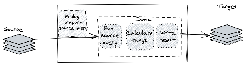
The first thing I try to do is try to figure out which of these steps takes the most of time.

Reading source data

You can time how long the source view calculation takes by recording how long it takes from the last line of Prolog tab to first record appearing in Data tab. Add something along the lines of

if (nCountRecords = 0); 
	we finished processing source, yay us; 
endif;

in the beginning of Data tab.

You can also export your source query to a csv file file and switch TI to read from it to ‘exclude’ the preparation time from TI time.

If this ‘preparation’ step takes a long time, there’s a few things to check:

• if it’s a SQL source – look at the query and aggregate, filter and narrow it down to the data you need. If it’s still slow – look at it’s execution plan and tweak it or pay your ‘database guy’ a visit (don’t forget to bring coffee and yummy pastries!)
• if it’s a cube view – check whether you’re getting MTQ on the source view construction. tm1top or PAA should show multiple worker threads for the query in the ‘source preparation stage’. There’s almost no reason why you shouldn’t see MTQ on a large enough source view (and you wouldn’t be looking to optimise a small view anyway), so check if it’s there. If you’re seeing an MTQ enabled source view preparation and it still takes a long time, then source cube rule is the issue and you should enable }StatsByRule and have a look at what takes long in more detail. And I’d need another post on what can happen there :)

Running calculations

Calculations themselves are quite rarely a bottleneck in my experience, unless:

• you’re looping through something for each cell in the source data, i.e. you’re allocating 1 source cell to a set of target elements. The reduce data volume comment applies here, it’s usually worth looking at trying to ‘tighten’ your loops if you can. A common approach is to ‘pre-create’ subsets for looping through in prolog that filter out anything you’d have to skip in a loop, i.e. you create a subset of products that have allocation % so that you don’t have to loop through all dimension
• Looking up values in some other cube. CellGetting rule driven value form the cube that is different to your source can cause a slowdown because you might be missing the caching of calculation results. Try commenting out CellGetN and if it is slowing the process down – try ‘caching’ it yourself by copying it to a static slice or measure
• trying to do the balance type calculation the wrong way :) this one is hard to generalise nicely, but if you’re doing balance or similar time-aware (i.e. stock) calculation in a TI and it’s slow – see if you can do everything in a single loop over a timeline without using source view to give you target time periods.
• you’re calling other TIs for each cell. TI ‘start time’ is non-negligeable (0.01-0.02s) and if you’re running one for every source cell, this startup time will be dragging the whole execution.

Writing the results

It’s easy to check whether writing is the bottleneck by commenting out the CellPut’s and CellIncrements (or diverting them to a text file) and re-running the process.

If you’re writing to a database table and it’s slow, try using file export & database bulk loading functionality or at least ‘batch’ your insert statements into a ‘largish’ query and use one ODBCOutput for multiple source cells. Each ODBCOutput opens a new transaction to a database, so opening one for each cell has a large performance impact.

If you’re writing to another cube and it’s slow, check whether you’re ‘re-firing’ feeders as you do that and if it’s the case, experiment with writing data to a text file and loading the file to the target cube. Another less common approach is to remove the target cube rule in prolog and put it back up in Epilog to make sure that you’re ‘bulk updating’ the feeders (be careful as this is a lock-intensive operation).